Structure refinement in PHENIX
phenix.refine is the general purpose crystallographic structure refinement program
Available features
- Coordinate refinement:
- Restrained / unrestrained individual
- Grouped (rigid body)
- LBFGS minimization, Simulated Annealing
- Selective removing of stereochemistry restraints
- Adding custom bonds and angles
- Atomic Displacement Parameters (ADP) refinement:
- Restrained individual isotropic, anisotropic, mixed
- Group isotropic (one isotropic B per selected model part)
- TLS
- comprehensive mode: combined TLS + individual or group ADP
- Occupancy refinement (any: individual, group, constrained for alternative conformations)
- Anomalous f' and f'' refinement
- Bulk solvent correction (flat model using a mask) and anisotropic scaling
- Multiple refinement and scale target functions: least-squares (ls), maximum-likelihood (ml), phased maximum-likelihood (mlhl)
- FFT and direct summation based refinement
- Various electron density map calculations (including likelihood-weighted)
- Simple structure factor calculation (with or without bulk solvent and scaling)
- Combined automatic ordered solvent building, update and refinement
- Complete model and data statistics (including twinning analysis, Wilson B calculation, stereo-chemistry statistics and much more)
- Automatic detection of NCS related copies and building NCS restraints
- Refinement using X-ray, neutron or both experimental data
- Complex refinement strategies in one run
- Refinement at subatomic resolution (approx. < 1.0 A) with IAS model
- Refinement with twinned data
Current limitations
- No omit maps calculation (use PHENIX wizards for this)
- TLS and individual anisotropic ADP cannot be refined at once for the same group
- Certain refinement strategies are not available for joint X-ray/neutron refinement
- No NCS constraints (restraints only)
- Atoms with anisotropic ADP in NCS groups
- No Simulated Annealing for selected fragments.
Remark on using amplitudes (Fobs) vs intensities (Iobs)
Although phenix.refine can read in both data types, intensities or amplitudes, internally it uses amplitudes in nearly all calculations. Both ways of doing refinement, with Iobs or Fobs, have their own slight advantages and disadvantages. To our knowledge there is no strong points to argue using one data type w.r.t. another.
phenix.refine organization
A refinement run in phenix.refine always consists of three main steps: reading in and processing of the data (model in PDB format, reflections in most known formats, parameters and optionally cif files with stereochemistry definitions), performing requested refinement protocols (bulk solvent and scaling, refinement of coordinates and B-factors, water picking, etc...) and finally writing out refined model, complete refinement statistics and electron density maps in various formats. The figure below illustrates these steps:
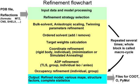
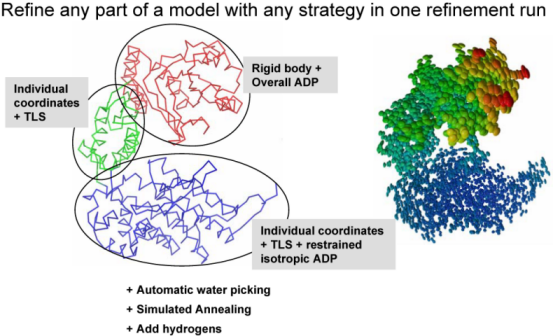
The second central step encompassing from bulk solvent correction and scaling to refinement of particular model parameters is called macro-cycles and repeated several times (3 by default). Multiple refinement scenario can be realized at this step and applied to any selected part of a model as illustrated at figure below:
Running phenix.refine
phenix.refine is run from the command line:
% phenix.refine <pdb-file(s)> <reflection-file(s)> <monomer-library-file(s)>
When you do this a number of things happen:
- The program automatically generates a ".eff" file which contains all of the parameters for the job (for example if you provided lysozyme.pdb the file lysozyme_refine_001.eff will be generated). This is the set of input parameters for this run.
- The program automatically interprets the reflection file(s). If there is an unambiguous choice of data arrays these will be used for the refinement. If there is a choice, you're given a message telling you how to select the arrays. Several reflection files can be provided, for example: one containing Fobs and another one with R-free flags.
- Once the data arrays are chosen, the program writes all of the data it will be using in the refinement to a new MTZ file, for example, lysozyme_refine_data.mtz. This makes it very easy to keep track of what you actually used in the refinement (instead of having the arrays spread across multiple files).
- At the end of refinement the program generates:
a new PDB file, with the refined model, called for example lysozyme_refine_001.pdb;
two maps: likelihood weighted mFo-DFc and 2mFo-DFc. These are in ASCII X-PLOR format. A reflection file with map coefficients is also generated for use in Coot or XtalView (e.g. lysozyme_refine_001_map_coeffs.mtz);
a new defaults file to run the next cycle of refinement, e.g. lysozyme_refine_002.def. This means you can run the next cycle of refinement by typing:
% phenix.refine lysozyme_refine_002.def
To get information about command line options type:
% phenix.refine --help
To have the program generate the default input parameters without running the refinement job (e.g. if you want to modify the parameters prior to running the job):
% phenix.refine --dry_run <pdb-file> <reflection-file(s)>
If you know the parameter that you want to change you can override it from the command line:
% phenix.refine data.hkl model.pdb xray_data.low_resolution=8.0 \
  simulated_annealing.start_temperature=5000
Note that you don't have to specify the full parameter name. What you specify on the command line is matched against all known parameters names and the best substring match is used if it is unique.
To rerun a job that was previously run:
% phenix.refine --overwrite lysozyme_refine_001.def
The --overwrite option allows the program to overwrite existing files. By default the program will not overwrite existing files - just in case this would remove the results of a refinement job that took a long time to finish.
To see all default parameters:
% phenix.refine --show-defaults=all
Giving parameters on the command line or in files
In phenix.refine parameters to control refinement can be given by the user on the command line:
% phenix.refine data.hkl model.pdb simulated_annealing=true
However, sometimes the number of parameters is large enough to make it difficult to type them all on the command line, for example:
% phenix.refine data.hkl model.pdb refine.adp.tls="chain A" \
  refine.adp.tls="chain B" main.number_of_macro_cycles=4 \
  xray_data.high_resolution=2.5 wxc_scale=3 wxu_scale=5 \
  output.prefix=my_best_model strategy=tls+individual_sites+individual_adp \
  simulated_annealing.start_temperature=5000
The same result can be achieved by using:
% phenix.refine data.hkl model.pdb custom_par_1.params
where the custom_par_1.params file contains the following lines:
refinement.refine.strategy=tls+individual_sites+individual_adp
refinement.refine.adp.tls="chain A"
refinement.refine.adp.tls="chain B"
refinement.main.number_of_macro_cycles=4
refinement.input.xray_data.high_resolution=2.5
refinement.target_weights.wxc_scale=3
refinement.target_weights.wxu_scale=5
refinement.output.prefix=my_best_model
refinement.simulated_annealing.start_temperature=5000
which can also be formatted by grouping the parameters under the relevant scopes (custom_par_2.params):
refinement.main {
   number_of_macro_cycles=4
}
refinement.input.xray_data.high_resolution=2.5
refinement.refine {
  strategy = *individual_sites \
              rigid_body \
             *individual_adp \
              group_adp \
             *tls \
              occupancies \
              group_anomalous \
              none
  adp {
    tls = "chain A"
    tls = "chain B"
  }
}
refinement.target_weights {
  wxc_scale=3
  wxu_scale=5
}
refinement.output.prefix=my_best_model
refinement.simulated_annealing.start_temperature=5000
and the refinement run will be:
% phenix.refine data.hkl model.pdb custom_par_2.params
The easiest way to create a file like the custom_par_2.params file is to generate a template file containing all parameters by using the command phenix.refine --show-defaults=all and then take the parameters that you want to use (and remove the rest).
Comments in parameter files
Use # for comments:
% phenix.refine data.hkl model.pdb comments_in_params_file.params
where comments_in_params_file.params file contains the lines:
refinement {
  refine {
    #strategy =  individual_sites rigid_body  individual_adp group_adp tls \
    #           occupancies group_anomalous *none
  }
  #main {
  #  number_of_macro_cycles = 1
  #}
}
refinement.target_weights.wxc_scale = 1.5
#refinement.input.xray_data.low_resolution=5.0
In this example the only parameter that is used to overwrite the defaults is target_weights.wxc_scale and the rest is commented.
Refinement scenarios
The refinement of atomic parameters is controlled by the strategy keyword. Those include:
- individual_sites (refinement of individual atomic coordinates)
- individual_adp   (refinement of individual atomic B-factors)
- group_adp        (group B-factors refinement)
- group_anomalous  (refinement of f' and f" values)
- tls              (TLS refinement = refinement of ADP through TLS parameters)
- rigid_body       (rigid body refinement)
- none             (bulk solvent and anisotropic scaling only)
Below are examples to illustrate the use of the strategy keyword as well as a few others.
Refinement with all default parameters
% phenix.refine data.hkl model.pdb
This will perform coordinate refinement and restrained ADP refinement. Three macrocycles will be executed, each consisting of bulk solvent correction, anisotropic scaling of the data, coordinate refinement (25 iterations of the LBFGS minimizer) and ADP refinement (25 iterations of the LBFGS minimizer). At the end the updated coordinates, maps, map coefficients, and statistics are written to files.
Refinement of coordinates
phenix.refine offers three ways of coordinate refinement:
- individual coordinate refinement using gradient-driven (LBFGS) minimization;
- individual coordinate refinement using simulated annealing (SA refinement);
- grouped coordinate refinement (rigid body refinement).
All types of coordinate refinement listed above can be used separately or combined all together in any combination and can be applied to any selected part of a model. For example, if a model contains three chains A, B and C, than it would require only one single refinement run to perform SA refinement and minimization for atoms in chain A, rigid body refinement with two rigid groups A and B, and refine nothing for chain C. Below we will illustrate this with several examples.
The default refinement includes a standard set of stereo-chemical restraints ( covalent bonds, angles, dihedrals, planarities, chiralities, non-bonded). The NCS restrains can be added as well. Completely unrestrained refinement is possible.
The total refinement target is defined as:
Etotal = wxc_scale * wxc * Exray + wc * Egeom
where: Exray is crystallographic refinement target (least-squares, maximum-likelihood, or any other), Egeom is the sum of restraints (including NCS if requested), wc is 1.0 by default and used to turn the restraints off, wxc ~ ratio of gradient's norms for geometry and X-ray targets as defined in (Adams et al, 1997, PNAS, Vol. 94, p. 5018), wc_scale is an 'ad hoc' scale found empirically to be ok for most of the cases.
Important to note:
When a refinement of coordinates (individual or rigid body) is run without using selections, then the coordinates of all atoms will be refined. Otherwise, if selections are used, the only coordinates of selected atoms will be refined and the rest will be fixed.
Using strategy=rigid_body or strategy=individual_sites will ask phenix.refine to refine only coordinates while other parameters (ADP, occupancies) will be fixed.
phenix.refine will stop if an atom at special position is included in rigid body group. The solution is to make a new rigid body group selection containing no atoms at special positions.
Rigid body refinement
phenix.refine implementation of rigid body refinement is very sophisticated and efficient (big convergence radius, one run, no need to cut off high-resolution data). We call this MZ protocol (multiple zones). The essence of MZ protocol is that the refinement starts with a few reflections selected in the lowest resolution zone and proceeds with gradually adding higher resolution reflections. Also, it almost constantly updates the mask and bulk solvent model parameters and this is crucial since the bulk solvent affects the low resolution reflections - exactly those the most important for success of rigid body refinement. The default set of the rigid body parameters is good for most of the cases and is normally not supposed to be changed.
One rigid body group (whatever is in the PDB file is refined as a single rigid body):
% phenix.refine data.hkl model.pdb strategy=rigid_body
Multiple groups (requires a basic knowledge of the PHENIX atom selection language, see below):
% phenix.refine data.hkl model.pdb strategy=rigid_body \
  sites.rigid_body="chain A" sites.rigid_body="chain B"
This will refine the chain A and chain B as two rigid bodies. The rest of the model will be kept fixed.
If one have many rigid groups, a lot of typing in the command line may not be convenient, so creating a parameter file rigid_body_selections, containing the following lines, may be a good idea:
refinement.refine.sites {
  rigid_body = chain A
  rigid_body = chain B
}
The command line will then be:
% phenix.refine data.hkl model.pdb strategy=rigid_body rigid_body_selections.params
Files like this can be created, for example, by copy-and-paste from the complete list of parameters (phenix.refine --show-defaults=all).
To switch from MZ protocol to traditional way of doing rigid body refinement (not recommended!):
% phenix.refine data.hkl model.pdb strategy=rigid_body rigid_body.number_of_zones=1 \
  rigid_body.high_resolution=4.0
Note that doing one zone refinement one need to cut the high-resolution data off at some arbitrary point around 3-5 A (depending on model size and data quality).
By default the rigid body refinement is run only the first macro-cycles. To switch from running rigid body refinement only once at the first macro-cycle to running it every macro-cycle:
% phenix.refine data.hkl model.pdb strategy=rigid_body rigid_body.mode=every_macro_cycle
To change the default number of lowest resolution reflections used to determine the first resolution zone to do rigid body refinement in it (for MZ protocol only):
% phenix.refine data.hkl model.pdb strategy=rigid_body \
  rigid_body.min_number_of_reflections=250
Decreasing this number may increase the convergence radius of rigid body refinement but small numbers may lead to refinement instability.
To change the number of zones for MZ protocol:
% phenix.refine data.hkl model.pdb strategy=rigid_body \
  rigid_body.number_of_zones=7
Increasing this number may increase the convergence radius of rigid body refinement at the cost of much longer run time.
Rigid body refinement can be combined with individual coordinates refinement in a smart way:
% phenix.refine data.hkl model.pdb strategy=rigid_body+individual_sites
this will perform 3 macro-cycles of individual coordinates refinement and the rigid body refinement will be performed only once at the first macro-cycle. More powerful combination for coordinates refinement is:
% phenix.refine data.hkl model.pdb strategy=rigid_body+individual_sites \
  simulated_annealing=true
this will do the same refinement as above plus the Simulated annealing at the second macro-cycle (see more options/examples for running SA in this document).
Refinement of individual coordinates
Refinement with Simulated Annealing:
% phenix.refine data.hkl model.pdb simulated_annealing=true \
  strategy=individual_sites
This will perform the Simulated Annealing refinement and LBFGS minimization for the whole model.
To change the start SA temperature:
% phenix.refine data.hkl model.pdb simulated_annealing=true \
  strategy=individual_sites simulated_annealing.start_temperature=10000
Since a SA run may take some time, there are several options defining of how many times the SA will be performed per refinement run. Run it only the first macro_cycle:
% phenix.refine data.hkl model.pdb simulated_annealing=true \
  strategy=individual_sites simulated_annealing.mode=first
or every macro-cycle:
% phenix.refine data.hkl model.pdb simulated_annealing=true \
  strategy=individual_sites simulated_annealing.mode=every_macro_cycle
or second and before the last macro-cycle:
% phenix.refine data.hkl model.pdb simulated_annealing=true \
strategy=individual_sites simulated_annealing.mode=second_and_before_last
Refinement with minimization (whole model):
% phenix.refine data.hkl model.pdb strategy=individual_sites
Refinement with minimization (selected part of model):
% phenix.refine data.hkl model.pdb strategy=individual_sites \
sites.individual="chain A"
This will refine the coordinates of atoms in chain A while keeping fixed the atomic coordinates in chain B.
To perform unrestrained refinement of coordinates (usually at ultra-high resolutions):
% phenix.refine data.hkl model.pdb strategy=individual_sites wc=0
This assigns the contribution of the geometry restraints target to zero. However, it is still calculated for statistics output.
Removing selected geometry restraints
In the example below:
% phenix.refine data.hkl model.pdb remove_restraints_selections.params
where remove_restraints_selections.params contains:
refinement {
  geometry_restraints.remove {
    angles = chain B
    dihedrals = name CA
    chiralities = all
    planarities = None
  }
}
the following restraints will be removed: angle for all atoms in chain B, dihedral for all involving CA atoms, all chirality. All planarity restraints will be preserved.
Refinement of atomic displacement parameters (commonly named as ADP or B-factors)
An ADP in phenix.refine is defined as a sum of three contributions:
Utotal = Ulocal + Utls + Ucryst
where Utotal is the total ADP, Ulocal reflects the local atomic vibration (also named as residual B) and Ucryst reflects global lattice vibrations. Ucryst is determined and refined at anisotropic scaling stage.
phenix.refine offers multiple choices for ADP refinement:
- individual isotropic, anisotropic or mixed ADP;
- grouped with one isotropic ADP per selected group;
- TLS.
All types of ADP refinement listed above can be used separately or combined all together in any combination (except TLS+individual anisotropic) and can be applied to any selected part of a model. For example, if a model contains six chains A, B, C, D, E and F than it would require only one single refinement run to perform refinement of:
- individual isotropic ADP for atoms in chain A,
- individual anisotropic ADP for atoms in chain B,
- grouped B with one B per residue for chain C,
- TLS refinement for chain D,
- TLS and individual isotropic refinement for chain E,
- TLS and grouped B refinement for chain F.
Below we will illustrate this with several examples.
Restraints are used for default ADP refinement of isotropic and anisotropic atoms. Completely unrestrained refinement is possible.
The total refinement target is defined as:
Etotal = wxu_scale * wxu * Exray + wu * Eadp
where: Exray is crystallographic refinement target (least-squares, maximum-likelihood, ...), Eadp is the ADP restraints term, wu is 1.0 by default and used to turn the restraints off, wxu and wc_scale are defined similarly to coordinates refinement (see Refinement of Coordinates paragraph).
It is important to keep in mind:
If a model was previously refined using TLS that means all atoms participating in TLS groups are reported in output PDB file as anisotropic (have ANISOU records). Now if a PDB file like this is submitted for default refinement then all atoms with ANISOU records will be refined as individual anisotropic which is most likely not desired.
When performing TLS refinement along with individual isotropic refinement of Ulocal, the restraints are applied to Ulocal and not to the total ADP (Ulocal+Utls).
When performing group B or TLS refinement only, no ADP restrains is used.
When ADP refinement is run without using selections then ADP for all atoms will be refined. Otherwise, if selections are used, the only ADP of selected atoms will be refined and the ADP of the rest will be unchanged.
If a TLS parametrization is used for a model previously refined with individual anisotropic ADP then normally an increase of R-factors is expected.
phenix.refine will stop if an atom at special position is included in TLS group. The solution is to make a new TLS group selection containing no atoms at special positions.
When refining TLS, the output PDB file always has the ANISOU records for the atoms involved in TLS groups. The anisotropic B-factor in ANISOU records is the total B-factor (B_tls + B_individual). The isotropic equivalent B-factor in ATOM records is the mean of the trace of the ANISOU matrix divided by 10000 and multiplied by 8*pi^2 and represents the isotropic equivalent of the total B-factor (B_tls + B_individual). To obtain the individual B-factors, one needs to compute the TLS component (B_tls) using the TLS records in the PDB file header and then subtract it from the total B-factors (on the ANISOU records).
Refining group isotropic B-factors
One B-factor per residue:
% phenix.refine data.hkl model.pdb strategy=group_adp
One isotropic B per selected group of atoms:
% phenix.refine data.hkl model.pdb strategy=group_adp \
  one_adp_group_per_residue=false adp.group="chain A" adp.group="chain B"
This will refine one isotropic B for chain A and one B for chain B.
The refinement of group isotropic B-factors in phenix.refine does not change the original distribution of B-factors within the group, that is the differences between B-factors for atoms withing the group remain constant while the only total component added to all atoms of given group is varied. The atoms with anisotropic ADP are allowed to be withing the group.
Refinement of individual ADP (isotropic, anisotropic)
By default atoms in a PDB file with ANISOU records are refined as anisotropic and atoms without ANISOU records are refined as isotropic. This behavior can be changed with appropriate keywords.
Default refinement of individual ADP:
% phenix.refine data.hkl model.pdb strategy=individual_adp
Note, atoms in input PDB file with ANISOU records will be refined as anisotropic and those without ANISOU - as isotropic.
Refinement of individual isotropic ADP for a model previously refined as anisotropic or TLS:
% phenix.refine data.hkl model.pdb strategy=individual_adp \
  adp.individual.isotropic=all
or equivalently:
% phenix.refine data.hkl model.pdb strategy=individual_adp \
  convert_to_isotropic=true
All anisotropic atoms in input PDB file will be converted to isotropic before the refinement starts. Obviously, this may raise the R-factors.
Refinement of individual anisotropic ADP for a model previously refined as isotropic:
% phenix.refine data.hkl model.pdb strategy=individual_adp \
  adp.individual.anisotropic="not element H"
This will refine all atoms as anisotropic except hydrogens.
Refinement of mixed model (some atoms are isotropic, some are anisotropic):
% phenix.refine data.hkl model.pdb strategy=individual_adp \
  adp.individual.anisotropic="chain A and not element H" \
  adp.individual.isotropic="chain B or element H"
In this example the atoms (except hydrogens if any) in chain A will be refined as anisotropic and the atoms in chain B (and hydrogens if any) will be refined as isotropic. Often, the ADP of water and hydrogens are desired to be refined as isotropic while the other atoms - as anisotropic:
% phenix.refine data.hkl model.pdb strategy=individual_adp \
  adp.individual.anisotropic="not water and not element H" \
  adp.individual.isotropic="water or element H"
Exactly the same command using slightly shorter selection syntax:
% phenix.refine data.hkl model.pdb strategy=individual_adp \
  adp.individual.anisotropic="not (water or element H)" \
  adp.individual.isotropic="water or element H"
To perform unrestrained individual ADP refinement (usually at ultra-high resolutions):
% phenix.refine data.hkl model.pdb strategy=individual_adp wu=0
This assigns the contribution of the ADP restraints target to zero. However, it is still calculated for statistics output.
TLS refinement
Refinement of TLS parameters only (whole model as one TLS group):
% phenix.refine data.hkl model.pdb strategy=tls
Refinement of TLS parameters only (multiple TLS group):
% phenix.refine data.hkl model.pdb strategy=tls tls_group_selections.params
where, similar to the rigid body or group B-factor refinement, the selection for TLS groups has been made in a user-created parameter file (tls_group_selections.params) as following:
refinement.refine.adp {
  tls = chain A
  tls = chain B
}
Alternatively, the selection for the TLS groups can be made from the command line (see rigid body refinement for an example).
Note: TLS parameters will be refined only for selected fragments. This, for example, will allow to not include the solvent molecules into the TLS groups.
More complete is to perform combined TLS and individual or grouped isotropic ADP refinement:
% phenix.refine data.hkl model.pdb strategy=tls+individual_adp
or:
% phenix.refine data.hkl model.pdb strategy=tls+group_adp
This will allow to model global (TLS) and local (individual) components of the total ADP and also compensate for the model parts where TLS parametrization doesn't suite well.
Occupancy refinement
By default, the occupancy refinement is selected (star in front of corresponding keyword: strategy = ... *occupancies ...). This does not mean that occupancies for all atoms will be refined. This just tells phenix.refine to automatically find which occupancies it will be refining ( based on input PDB file). Here are the possible scenarios:
- if no selections are provided (refine.occupancies.individual=None and refine.occupancies.group=None) then phenix.refine by default will refine individual occupancies for atoms that have partial occupancy values in input PDB file (except zeros) and it will perform group constrained occupancy refinement for all atoms in alternative conformations. Occupancies of all other atoms will be fixed.
- If selections are provided (refine.occupancies.individual=atom_selection or refine.occupancies.group=atom_selection) then the selected atoms will be added to the list of atoms defined above (atoms with partial occupancies or those in alternative conformations). See this document for examples of atom_selection syntax.
Refinement of occupancies only:
% phenix.refine data.hkl model.pdb strategy=occupancies
This will only refine occupancies for atoms in alternative conformations or for atoms having partial occupancies (other model parameters, like B-factors or coordinates will be fixed).
Refine occupancies of water in addition to atoms with partial occupancies and those in alternative conformations:
% phenix.refine data.hkl model.pdb \
  refine.occupancies.individual="water"
Refine one occupancy factor per selected group of atoms (group occupancy refinement):
% phenix.refine data.hkl model.pdb strategy=occupancies \
  refine.occupancies.group="chain A and resseq 1" \
  refine.occupancies.group="chain B and resseq 3"
this will refine two occupancy factors: one for residue number 1 in chain A and another one for residue number 3 in chain B. This feature is frequently used for refinement of occupancies of partially occupied ligands. Additionally, the partial occupancies and those for atoms in alternative conformations will be refined since they are selected automatically by default.
f' and f'' refinement
If the structure contains anomalous scatterers (e.g. Se in a SAD or MAD experiment), and if anomalous data are available, it is possible to refine the dispersive (f') and anomalous (f") scattering contributions (see e.g. Ethan Merritt's tutorial for more information). In phenix.refine, each group of scatterers with common f' and f" values is defined via an anomalous_scatterers scope, e.g.:
refinement.refine.anomalous_scatterers {
  group {
    selection = name BR
    f_prime = 0
    f_double_prime = 0
    refine = *f_prime *f_double_prime
  }
}
NOTE: The refinement of the f' and f" values is carried out only if group_anomalous is included under refine.strategy! Otherwise the values are simply used as specified but not refined. So the refinement run with the parameters above included into group_anomalous_1.params:
% phenix.refine model.pdb data_anom.hkl group_anomalous_1.params \
  strategy=individual_sites+individual_adp+group_anomalous
If required, multiple scopes can be specified, one for each unique pair of f' and f" values. These values are assigned to all selected atoms (see below for atom selection details). Often it is possible to start the refinement from zero. If the refinement is not stable, it may be necessary to start from better estimates, or even to fix some values. For example (file group_anomalous_2.params):
refinement.refine.anomalous_scatterers {
  group {
    selection = name BR
    f_prime = -5
    f_double_prime = 2
    refine = f_prime *f_double_prime
  }
}

% phenix.refine model.pdb data_anom.hkl group_anomalous_2.params \
  strategy=individual_sites+individual_adp+group_anomalous
Here f' is fixed at -5 (note the missing * in front of f_prime in the refine definition), and the refinement of f" is initialized at 2.
The phenix.form_factor_query command is available for obtaining estimates of f' and f" given an element type and a wavelength, e.g.:
% phenix.form_factor_query element=Br wavelength=0.8

Information from Sasaki table about Br (Z = 35) at 0.8 A
fp:  -1.0333
fdp: 2.9928
Run without arguments for usage information:
% phenix.form_factor_query
Using NCS restraints in refinement
phenix.refine can find NCS automatically or use NCS selections defined by the user. Gaps in selected sequences are allowed - a sequence alignment is performed to detect insertions or deletions. We recommend to check the automatically detected or adjusted NCS groups.
Refinement with user provided NCS selections.
Create a ncs_groups.params file with the NCS selections:
refinement.ncs.restraint_group {
  reference = chain A resid 1:4
  selection = chain B and resid 1:3
  selection = chain C
}
refinement.ncs.restraint_group {
  reference = chain E
  selection = chain F
}
Specify ncs_groups.params as an additional input when running phenix.refine:
% phenix.refine data.hkl model.pdb ncs_groups.params main.ncs=True
This will perform the default refinement round (individual coordinates and B-factors) using NCS restraints on coordinates and B-factors.
Note: user specified NCS restraints in ncs_groups.params can be modified automatically if better selection is found. To disable this potential automatic adjustment:
% phenix.refine data.hkl model.pdb ncs_groups.params main.ncs=True \
  ncs.find_automatically=False
Automatic detection of NCS groups:
% phenix.refine data.hkl model.pdb main.ncs=True
This will perform the default refinement round (individual coordinates and B-factors) using NCS restraints automatically created based on input PDB file.
Water picking
phenix.refine has very efficient and fully automated protocol for water picking and refinement. One run of phenix.refine is normally necessary to locate waters, refine them, select good ones, add new and refine again, repeating the whole process multiple times.
Normally, the default parameter settings are good for most cases:
% phenix.refine data.hkl model.pdb ordered_solvent=true
This will perform new water picking, analysis of existing waters and refinement of individual coordinates and B-factors for both, macromolecule and waters. Several cycles will be performed allowing sorting out of spurious waters and refinement of well placed ones.
Water picking can be combined with all others protocols, like simulated annealing, TLS refinement, etc. Some useful commands are:
Perform water picking every macro-cycle.
By default, water picking starts after a half of macro-cycles is done:
% phenix.refine data.hkl model.pdb ordered_solvent=true \
  ordered_solvent.mode=every_macro_cycle
Remove water only (based on specified criteria):
% phenix.refine data.hkl model.pdb ordered_solvent=true \
  ordered_solvent.mode=filter_only
The following run illustrates the use of some important parameters:
% phenix.refine data.hkl model.pdb ordered_solvent=true solvent.params
where the parameter file solvent.params contains:
refinement {
  ordered_solvent {
    low_resolution = 2.8
    b_iso_min = 1.0
    b_iso_max = 50.0
    b_iso = 25.0
    primary_map_type = mFobs-DFmodel
    primary_map_cutoff = 3.0
    secondary_map_type = 2mFobs-DFmodel
  }
  peak_search {
    map_next_to_model {
      min_model_peak_dist = 1.8
      max_model_peak_dist = 6.0
      min_peak_peak_dist = 1.8
    }
  }
}
This will skip water picking if the resolution of data is lower than 2.8A, it will remove waters with B < 1.0 or B > 50.0 A**2 or occupancy different from 1 or peak height at mFo-DFc map lower then 3 sigma. It will not select or will remove existing water if water-water or water-macromolecule distance is less than 1.8A or water-macromolecule distance is greater than 6.0 A. The initial occupancies and B-factors of newly placed waters will be 1.0 and 25.0 correspondingly. If b_either = None, then b_iso will be the mean atomic B-factor.
Hydrogens in refinement
phenix.refine offers two possibilities for handling of hydrogen atoms:
- riding model;
- complete refinement of H (H atoms will be refined as other atoms in the model)
Although the contribution of hydrogen atoms to X-ray scattering is weak (at high resolution) or negligible (at lower resolutions), the H atoms still present in real structures irrespective the data quality. Including them as riding model makes other model atoms aware of their positions and hence preventing non-physical (bad) contacts at no cost in terms of refinable parameters (= no risk of overfitting).
At subatomic resolution (approx. < 1.0 A) X-ray refinement or refinement using neutron data the parameters of H atoms may be refined as for other heavier atoms.
Below are some useful commands:
To add hydrogens to a model one need to run the Reduce program:
% phenix.reduce model.pdb > model_h_added.pdb
Once hydrogens added to a model, by default they will be refined as riding model:
% phenix.refine model.pdb data.hkl
It is possible to refine individual parameters for H atoms (if neutron data is used or at ultra-high resolution):
% phenix.refine model.pdb data.hkl hydrogens.refine=individual
To refine individual coordinates and ADP of H atoms:
% phenix.refine model.pdb data.hkl hydrogens.refine=individual
To remove hydrogens from a model:
% phenix.pdbtools model.pdb remove="element H"
We strongly recommend to not remove hydrogen atoms after refinement since it will make the refinement statistics (R-factors, etc...) unreproducible without repeating exactly the same refinement protocol.
Normally, phenix.reduce is used to add hydrogens. However, it may happen that phenix.reduce fails to add H to certain ligands. In this case phenix.elbow can be used to add hydrogens:
% phenix.elbow --final-geometry=model.pdb --residue=MAN --output=model_h
An output PDB file called model_h.pdb will contain the original ligand MAN with all hydrogen atoms added.
Refinement using twinned data
phenix.refine can handle the refinement of hemihedrally twinned data (two twin domains). Least square twin refinement can be carried out using the following commands line instructions:
% phenix.refine data.hkl model.pdb twin_law="-k,-h,-l"
The twin law (in this case -k,-h,-l) can be obtained from phenix.xtriage. If more than a single twin law is possible for the given unit cell and space group, using phenix.twin_map_utils might give clues which twin law is the most likely candidate to be used in refinement.
Correcting maps for anisotropy might be useful:
% phenix.refine data.hkl model.pdb twin_law="-k,-h,-l" \
  detwin.map_types.aniso_correct=true
The detwinning mode is auto by default: it will perform algebraic detwinning for twin fraction below 40%, and detwinning using proportionality rules (SHELXL style) for fractions above 40%.
An important point to stress is that phenix.refine will only deal properly with twinning that involves two twin domains.
Neutron and joint X-ray and neutron refinement
Refinement using neutron data requires having H or/and D atoms added to the model. Use Reduce program to add all potential H atoms:
% phenix.reduce model.pdb > model_h.pdb
Currently, adding D atoms will require editing of model_h.pdb file to replace H with D where necessary.
Running refinement with neutron data only:
% phenix.refine data.hkl model.pdb main.scattering_table=neutron
this will tell phenix.refine that the data in data.hkl file is coming from neutron scattering experiment and the appropriate scattering factors will be used in all calculations. All the examples and phenix.refine functionality presented in this document are valid and compatible with using neutron data.
Using X-ray and neutron data simultaneously (joint X/N refinement).
phenix.refine allows simultaneous use of both data sets, X-ray and neutron. The data sets are allowed to have different number of reflections and be collected at different resolutions.
The only requirement (that is not enforced by the program but is the user's responsibility) is that both data sets have to be collected at the same temperature from same crystals (or grown in identical conditions, having identical space groups and unit cell parameters).
phenix.refine model.pdb data_xray.hkl neutron_data.file_name=data_neutron.hkl input.xray_data.labels=FOBSx input.neutron_data.labels=FOBSn
Optimizing target weights
phenix.refine uses automatic procedure to determine the weights between X-ray target and stereochemistry or ADP restraints. To optimize these weights (that is to find those resulting in lowest Rfree factors):
% phenix.refine data.hkl model.pdb optimize_wxc=true optimize_wxu=true
where optimize_wxc will turn on the optimization of X-ray/stereochemistry weight and optimize_wxu will turn on the optimization of X-ray/ADP weight. Note that this could be very slow since the procedure involves a grid search over an array of weights-candidates. It could be a good idea to run this overnight for a final model tune up.
Refinement at high resolution (higher than approx. 1.0 Angstrom)
Guidelines for structure refinement at high resolution:
make sure the model contains hydrogen atoms. If not, phenix.reduce can be used to add them:
% phenix.reduce model.pdb > model_h.pdbBy default, phenix.refine will refine positions of H atoms as riding model (H atom will exactly follow the atom it is attached to). Note that phenix.refine can also refine individual coordinates of H atoms (can be used for small molecules at ultra-high resolutions or for refinement against neutron data). This is governed by hydrogens.refine = individual *riding keyword and the default is to use riding model. hydrogens.refine defines how hydrogens' B-factors are refined (default is to refine one group B for all H atoms). At high resolution one should definitely try to use one_b_per_molecule or even individual choice (resolution permitting). Similar strategy should be used for refinement of H's occupancies, hydrogens.refine_occupancies keyword.
most of the atoms should be refined with anisotropic ADP. Exceptions could be model parts with high B-factors), atoms in alternative conformations, hydrogens and solvent molecules. However, at resolutions higher than 1.0A it's worth of trying to refine solvent with anisotropic ADP.
it is a good idea to constantly monitor the existing solvent molecules and check for new ones by using ordered_solvent=true keyword. If it's decided to refine waters with anisotropic ADP then make sure that the newly added ones are also anisotropic; use ordered_solvent.new_solvent=anisotropic (default is isotropic). One can also ask phenix.refine to refine occupancies of water: ordered_solvent.refine_occupancies=true (default is False).
at high resolution the alternative conformations can be visible for more than 20% of residues. phenix.refine automatically recognizes atoms in alternative conformations (based on PDB records) and by default does constrained refinement of occupancies for these atoms. Please note, that phenix.refine does not build or create the fragments in alternative conformations; the atoms in alternative conformations should be properly defined in input PDB file (using conformer identifiers) (if actually found in a structure).
the default weights for stereochemical and ADP restraints are most likely too tight at this resolution, so most likely the corresponding values need to be relaxed. Use wxc_scale and wxu_scale for this; lower values, like 1/2, 1/3, 1/4, ... etc of the default ones should be tried. phenix.refine allows automatically optimize these values ( optimize_wxc=True and optimize_wxu=True), however this is a very slow task so it may be considered for an over night run or even longer. At ultra-high resolutions (approx. 0.8A or higher) a complete unrestrained refinement should be definitely tried out for well ordered parts of the model (single conformations, low B-factors).
at ultra-high resolution the residual maps show the electron density redistribution due to bonds formation as density peaks at interatomic bonds. phenix.refine has specific tools to model this density called IAS models (Afonine et al, Acta Cryst. (2007). D63, 1194-1197).
This example illustrates most of the above points:
% phenix.refine model_h.pdb data.hkl high_res.params
where the file high_res.params contains following lines (for more parameters under each scope look at complete list of parameters):
refinement.main {
  number_of_macro_cycles = 5
  ordered_solvent=true
}
refinement.refine {
  adp {
    individual {
      isotropic = element H
      anisotropic = not element H
    }
  }
}
refinement.target_weights {
  wxc_scale = 0.25
  wxu_scale = 0.3
}
refinement {
  ordered_solvent {
    mode = auto filter_only *every_macro_cycle
    new_solvent =  isotropic *anisotropic
    refine_occupancies = True
  }
}
In the example above phenix.refine will perform 5 macro-cycles with ordered solvent update (add/remove) every macro-cycles, all atoms including newly added water will be refined with anisotropic B-factors (except hydrogens), riding model will be used for positional refinement of H atoms, one occupancy and isotropic B-factor will be refined per all hydrogens within a residue, occupancies of waters will be refined as well, the default stereochemistry and ADP restraints weights are scaled down by the factors of 0.25 and 0.3 respectively. If starting model is far enough from the "final" one, more macro-cycles may be required (than 5 used in this example).
Examples of frequently used refinement protocols, common problems
Starting refinement from high R-factors:
% phenix.refine data.hkl model.pdb ordered_solvent=true main.number_of_macro_cycles=10 \
  simulated_annealing=true strategy=rigid_body+individual_sites+individual_adp \
Depending on data resolution, refinement of individual ADP may be replaced with grouped B refinement:
% phenix.refine data.hkl model.pdb ordered_solvent=true simulated_annealing=true \
  strategy=rigid_body+individual_sites+group_adp main.number_of_macro_cycles=10
Adding TLS refinement may be a good idea. Note, unlike other programs, phenix.refine does not require "good model" for doing TLS refinement; TLS refinement is always stable in phenix.refine (please report if noticed otherwise):
% phenix.refine data.hkl model.pdb ordered_solvent=true simulated_annealing=true \
  strategy=rigid_body+individual_sites+individual_adp+tls main.number_of_macro_cycles=10
If NCS is present - once can use it:
% phenix.refine data.hkl model.pdb ordered_solvent=true simulated_annealing=true \
  strategy=rigid_body+individual_sites+individual_adp+tls main.ncs=true \
  main.number_of_macro_cycles=10 tls_group_selections.params \
  rigid_body_selections.params
where tls_groups_selections.txt, rigid_body_groups_selections.txt are the files TLS and rigid body groups selections, NCS will be determined automatically from input PDB file. See this document for details on how specify these selections.
Note: in these four examples above we re-defined the default number of refinement macro-cycles from 3 to 10, since a start model with high R-factors most likely requires more cycles to become a good one. Also in these examples, the rigid body refinement will be run only once at first macro-cycle, the water picking will start after half of macro-cycles is done (after 5th), the SA will be done only twice - the first and before the last macro-cycles. Even though it is requested, the water picking may not be performed if the resolution is too low. All these default behaviors can be changed: see parameter's help for more details.
The last command looks too long to type it in the command line. Look this document for an example of how to make it like this:
% phenix.refine data.hkl model.pdb custom_par_1.params
- Refinement at "higher than medium" resolution - getting anisotropic.
Refining at higher resolution one may consider:
- At resolutions around 1.8 ... 1.7 A or higher it is a good idea to try refinement of anisotropic ADP for atoms at well ordered parts of the model. Well ordered parts can be identified by relatively small isotropic B-factors ~5-20A**2 of so.
- The riding model for H atoms should be used.
- Loosing stereochemistry and ADP restraints.
- Re-thing using the NCS (if present): it may turn out to be enough of data to not use NCS restrains. Try both, with and without NCS, and based on R-free vales decide the strategy.
Supposing the H atoms were added to the model, below is an example of what may want to do at higher resolution:
% phenix.refine data.hkl model.pdb adp.individual.anisotropic="resid 1-2 and not element H" \
  adp.individual.isotropic="not (resid 1-2 and not element H)" wxc_scale=2 wxu_scale=2
In the command above phenix.refine will refine the ADP of atoms in residues from 1 to 2 as anisotropic, the rest (including all H atoms) will be isotropic, the X-ray target contribution is increased for both, coordinate and ADP refinement. IMPORTANT: Please make note of the selection used in the above command: selecting atoms in residues 1 and 2 to be refined as anisotropic, one need to exclude hydrogens, which should be refined as isotropic.
Stereochemistry looks too tightly / loosely restrained, or gap between R-free and R-work seems too big: playing with restraints contribution.
Although the automatic calculation of weight between X-ray and stereochemistry or ADP restraint targets is good for most of cases, it may happen that rmsd deviations from ideal bonds length or angles are looking too tight or loose ( depending on resolution). Or the difference between R-work and R-free is too big (significantly bigger than approx. 5%). In such cases one definitely need to try loose or tighten the restraints. Hers is how for coordinates refinement:
% phenix.refine data.hkl model.pdb wxc_scale=5
The default value for wxc_scale is 0.5. Increasing wxc_scale will make the X-ray target contribution greater and restraints looser. Note: wxc_scale=0 will completely exclude the experimental data from the refinement resulting in idealization of the stereochemistry. For stereochemistry idealization use the separate command:
% phenix.geometry_minimization model.pdb
To see the options type:
% phenix.geometry_minimization --help
To play with ADP restraints contribution:
% phenix.refine data.hkl model.pdb wxu_scale=3
The default value for wxu_scale is 1.0. Increasing wxu_scale will make the X-ray target contribution greater and therefore the B-factors restraints weaker.
Also, one can completely ignore the automatically determined weights (for both, coordinates and ADP refinement) and use specific values instead:
% phenix.refine data.hkl model.pdb fix_wxc=15.0
The refinement target will be: Etotal = 15.0 * Exray + Egeom
Similarly for ADP refinement:
% phenix.refine data.hkl model.pdb fix_wxu=25.0
The refinement target will be: Etotal = 25.0 * Exray + Eadp
Having unknown to phenix.refine item in PDB file (novel ligand, etc...).
phenix.refine uses the CCP4 Monomer Library as the source of stereochemical information for building geometry restraints and reposting statistics.
If phenix.refine is unable to match an item in input PDB file against the Monomer Library it will stop with "Sorry" message explaining what to do and listing the problem atoms. If this happened, it is necessary to obtain a cif file (parameter file, describing unknown molecule) by either making it manually or having eLBOW program to generate it:
phenix.elbow model.pdb --do-all --output=all_ligands
this will ask eLBOW to inspect the model_new.pdb file, find all unknown items in it and create one cif file for them all_ligands.cif. Alternatively, one can specify a three-letters name for the unknown residue:
phenix.elbow model.pdb --residue=MAN --output=man
Once the cif file is created, the new run of phenix.refine will be:
phenix.refine model.pdb data.pdb man.cif
Consult eLBOW documentation for more details.
Useful options
Changing the number of refinement cycles and minimizer iterations
% phenix.refine data.hkl model.pdb main.number_of_macro_cycles=5 \
  main.max_number_of_iterations=20
Creating R-free flags (if not present in the input reflection files)
% phenix.refine data.hkl model.pdb xray_data.r_free_flags.generate=True
It is important to understand that reflections selected for test set must be never used in any refinement of any parameters. If the newly selected test reflections were used in refinement before then the corresponding R-free statistics will be wrong. In such case "refinement memory" removal procedure must be applied to recover proper statistics.
To change the default maximal number of test flags to be generated and the fraction:
% phenix.refine data.hkl model.pdb xray_data.r_free_flags.generate=True \
  xray_data.r_free_flags.fraction=0.05 xray_data.r_free_flags.max_free=500
Specify the name for output files
% phenix.refine data.hkl model.pdb output.prefix=lysozyme
Reflection output
At the end of refinement a file with Fobs, Fmodel, Fcalc, Fmask, FOM, R-free_flags can be written out (in MTZ format):
% phenix.refine data.hkl model.pdb export_final_f_model=mtz
To output the reflections in CNS reflection file format:
% phenix.refine data.hkl model.pdb export_final_f_model=cns
Note: Fmodel is the total model structure factor including all scales:
Fmodel = scale_k1 * exp(-h*U_overall*ht) * (Fcalc + k_sol * exp(-B_sol*s^2) * Fmask)
Setting the resolution range for the refinement
% phenix.refine data.hkl model.pdb xray_data.low_resolution=15.0 xray_data.high_resolution=2.0
Bulk solvent correction and anisotropic scaling
By default phenix.refine always starts with bulk solvent modeling and anisotropic scaling. Here is the list of command that may be of use in some cases:
Perform bulk-solvent modeling and anisotropic scaling only:
% phenix.refine data.hkl model.pdb strategy=none
Bulk-solvent modeling only (no anisotropic scaling):
% phenix.refine data.hkl model.pdb strategy=none bulk_solvent_and_scale.anisotropic_scaling=false
Anisotropic scaling only (no bulk-solvent modeling):
% phenix.refine data.hkl model.pdb strategy=none bulk_solvent_and_scale.bulk_solvent=false
Turn off bulk-solvent modeling and anisotropic scaling:
% phenix.refine data.hkl model.pdb main.bulk_solvent_and_scale=false
Fixing bulk-solvent and anisotropic scale parameters to user defined values:
% phenix.refine data.hkl model.pdb bulk_solvent_and_scale.params
where bulk_solvent_and_scale.params is the file containing these lines:
refinement {
  bulk_solvent_and_scale {
    k_sol_b_sol_grid_search = False
    minimization_k_sol_b_sol = False
    minimization_b_cart = False
    fix_k_sol = 0.45
    fix_b_sol = 56.0
    fix_b_cart {
      b11 = 1.2
      b22 = 2.3
      b33 = 3.6
      b12 = 0.0
      b13 = 0.0
      b23 = 0.0
    }
  }
}
Mask parameters:
Bulk solvent modeling involves the mask calculation. There are three principal parameters controlling it: solvent_radius, shrink_truncation_radius and grid_step_factor. Normally, these parameters are not supposed to be changed but can be changed:
% phenix.refine data.hkl model.pdb refinement.mask.solvent_radius=1.0 \
  refinement.mask.shrink_truncation_radius=1.0 refinement.mask.grid_step_factor=3
If one wants to gain some more drop in R-factors (somewhere between 0.0 and 1.0%) it is possible to run fairly time consuming (depending on structure size and resolution) procedure of mask parameters optimization:
% phenix.refine data.hkl model.pdb optimize_mask=true
This will perform the grid search for solvent_radius and shrink_truncation_radius and select the values giving the best R-factor.
By default phenix.refine adds isotropic component of overall anisotropic scale matrix to atomic B-factors, leaving the trace of overall anisotropic scale matrix equals to zero. This is the reason why one can observe the ADP changed even though the only anisotropic scaling was done and no ADP refinement performed.
Default refinement with user specified X-ray target function
Refinement with least-squares target:
% phenix.refine data.hkl model.pdb main.target=ls
Refinement with maximum-likelihood target (default):
% phenix.refine data.hkl model.pdb main.target=ml
Refinement with phased maximum-likelihood target:
% phenix.refine data.hkl model.pdb main.target=mlhl
If phenix.refine finds Hendrickson-Lattman coefficients in input reflection file, it will automatically switch to mlhl target. To disable this:
% phenix.refine data.hkl model.pdb main.use_experimental_phases=false
Modifying the initial model before refinement starts
phenix.refine offers several options to modify input model before refinement starts:
shaking of coordinates (adding a random shift to coordinates):
% phenix.refine data.hkl model.pdb sites.shake=0.3
rotation-translation shift of coordinates:
% phenix.refine data.hkl model.pdb sites.rotate="1 2 3" sites.translate="4 5 6"
shaking of occupancies:
% phenix.refine data.hkl model.pdb occupancies.randomize=true
shaking of ADP:
% phenix.refine data.hkl model.pdb adp.randomize=true
shifting of ADP (adding a constant value):
% phenix.refine data.hkl model.pdb adp.shift_b_iso=10.0
scaling of ADP (multiplying by a constant value):
% phenix.refine data.hkl model.pdb adp.scale_adp=0.5
setting a value to ADP:
% phenix.refine data.hkl model.pdb adp.set_b_iso=25
converting to isotropic:
% phenix.refine data.hkl model.pdb adp.convert_to_isotropic=true
converting to anisotropic:
% phenix.refine data.hkl model.pdb adp.convert_to_anisotropic=true \
  modify_start_model.selection="not element H"
When converting atoms into anisotropic, it is important to make sure that hydrogens (if present in the model) are not converted into anisotropic.
By default, the specified manipulations will be applied to all atoms. However, it is possible to apply them to only selected atoms:
% phenix.refine data.hkl model.pdb adp.set_b_iso=25 modify_start_model.selection="chain A"
To write out the modified model (without any refinement), add: main.number_of_macro_cycles=0, e.g.:
% phenix.refine data.hkl model.pdb adp.set_b_iso=25 \
  main.number_of_macro_cycles=0
All the commands listed above plus some more are available from phenix.pdbtools utility which in fact is used internally in phenix.refine to perform these manipulations. For more information on phenix.pdbtools type:
% phenix.pdbtools --help
Documentation on phenix.pdbtools is also available.
Refinement using FFT or direct structure factor calculation algorithm
% phenix.refine data.hkl model.pdb \
  structure_factors_and_gradients_accuracy.algorithm=fft
or:
% phenix.refine data.hkl model.pdb \
  structure_factors_and_gradients_accuracy.algorithm=direct
Ignoring test (free) flags in refinement
Sometimes one need to use all reflections ("work" and "test") in the refinement; for example, at very low resolution where each single reflection counts, or at subatomic resolution where the risk of overfitting is very low. In the example below all the reflections are used in the refinement:
% phenix.refine data.hkl model.pdb xray_data.r_free_flags.ignore_r_free_flags=true
Note: 1) the corresponding statistics (R-factors, ...) will be identical for "work" and "test" sets; 2) it is still necessary to have test flags presented in input reflection file (or automatically generated by phenix.refine).
Using phenix.refine to calculate structure factors
The total structure factor used in phenix.refine nearly in all calculations is defined as:
Fmodel = scale_k1 * exp(-h*U_overall*ht) * (Fcalc + k_sol * exp(-B_sol*s^2) * Fmask)
Calculate Fcalc from atomic model and output in MTZ file (no solvent modeling or scaling):
% phenix.refine data.hkl model.pdb main.number_of_macro_cycles=0 \
  main.bulk_solvent_and_scale=false export_final_f_model=mtz
Calculate Fcalc from atomic model including bulk solvent and all scales:
% phenix.refine data.hkl model.pdb main.number_of_macro_cycles=1 \
  strategy=none export_final_f_model=mtz
To output CNS/Xplor formatted reflection file:
% phenix.refine data.hkl model.pdb main.number_of_macro_cycles=1 \
  strategy=none export_final_f_model=cns
Resolution limits can be applied:
% phenix.refine data.hkl model.pdb main.number_of_macro_cycles=1 \
  strategy=none xray_data.low_resolution=15.0 xray_data.high_resolution=2.0
Note:
- The number of calculated structure factors will the same as the number of observed data (Fobs) provided in the input reflection files or less since resolution and sigma cutoffs may be applied to Fobs or some Fobs may be automatically removed by outliers detection procedure.
- The set of calculated structure factors has the same completeness as the set of provided Fobs.
Scattering factors
There are four choices for the scattering table to be used in phenix.refine:
- wk1995: Waasmaier & Kirfel table;
- it1992: International Crystallographic Tables (1992)
- n_gaussian: dynamic n-gaussian approximation
- neutron: table for neutron scattering
The default is n_gaussian. To switch to different table:
% phenix.refine data.hkl model.pdb main.scattering_table=neutron
Suppressing the output of certain files
The following command will tell phenix,refine to not write .eff, .geo, .def, maps and map coefficients files:
% phenix.refine data.hkl model.pdb write_eff_file=false write_geo_file=false \
  write_def_file=false write_maps=false write_map_coefficients=false
The only output will be: .log and .pdb files.
Random seed
To change random seed:
% phenix.refine data.hkl model.pdb main.random_seed=7112384
The results of certain refinement protocols, such as restrained refinement of coordinates (with SA or LBFGS minimization), are sensitive to the random seed. This is because: 1) for SA the refinement starts with random assignment of velocities to atoms; 2) the X-ray/geometry target weight calculation involves model shaking with some Cartesian dynamics. As result, running such refinement jobs with exactly the same parameters but different random seeds will produce different refinement statistics. The author's experience includes the case where the difference in R-factors was about 2.0% between two SA runs.
Also, this opens a possibility to perform multi-start SA refinement to create an ensemble of slightly different models in average but sometimes containing significant variations in certain parts.
Electron density maps
By phenix.refine outputs two likelihood-weighted maps: 2mFo-DFc and mFo-DFc. The user can also choose between likelihood-weighted and regular maps with any specified coefficients, for example: 2mFo-DFc, 2.7mFo-1.3DFc, Fo-Fc, 3Fo-2Fc. The result is output as ASCII X-PLOR format. A reflection file with map coefficients is also generated for use in Coot or XtalView. The example below illustrates the main options:
% phenix.refine data.hkl model.pdb map.params
where map.params contains:
refinement {
  electron_density_maps {
    map {
      mtz_label_amplitudes = 2FOFCWT
      mtz_label_phases = PH2FOFCWT
      likelihood_weighted = True
      obs_factor = 2
      calc_factor = 1
    }
    map {
      mtz_label_amplitudes = FOFCWT
      mtz_label_phases = PHFOFCWT
      likelihood_weighted = True
      obs_factor = 1
      calc_factor = 1
    }
    map {
      mtz_label_amplitudes = 3FO2FCWT
      mtz_label_phases = PH3FO2FCWT
      likelihood_weighted = False
      obs_factor = 3
      calc_factor = 2
    }
    grid_resolution_factor = 1/4.
    region = *selection cell
    atom_selection = name CA or name N or name C
    apply_sigma_scaling = False
    apply_volume_scaling = True
  }
}
This will output three map files containing mFo-DFc, 2mFo-DFc and 3Fo-2Fc maps. All maps will be in absolute scale (in e/A**3). The map finess will be (data resolution)*grid_resolution_factor and the map will be output around main chain atoms. If atom_selection is set to None or all then map will be computed for all atoms. The corresponding MTZ file will also contain the map coefficients for these three maps.
Refining with anomalous data (or what phenix.refine does with Fobs+ and Fobs-).
The way phenix.refine uses Fobs+ and Fobs- is controlled by xray_data.force_anomalous_flag_to_be_equal_to parameter.
Here are 3 possibilities:
Default behavior: phenix.refine will use all Fobs: Fobs+ and Fobs- as independent reflections:
% phenix.refine model.pdb data_anom.hkl
phenix.refine will generate missing Bijvoet mates and use all Fobs+ and Fobs- as independent reflections if:
% phenix.refine model.pdb data_anom.hkl xray_data.force_anomalous_flag_to_be_equal_to=true
phenix.refine will merge Fobs+ and Fobs-, that is instead of two separate Fobs+ and Fobs- it will use one value F_mean = (Fobs+ + Fobs-)/2 if:
% phenix.refine model.pdb data_anom.hkl xray_data.force_anomalous_flag_to_be_equal_to=false
Look this documentation to see how to use and refine f' and f''.
Rejecting reflections by sigma
Reflections can be rejected by sigma cutoff criterion applied to amplitudes Fobs <= sigma_fobs_rejection_criterion * sigma(Fobs):
% phenix.refine model.pdb data_anom.hkl xray_data.sigma_fobs_rejection_criterion=2
or/and intensities Iobs <= sigma_iobs_rejection_criterion * sigma(Iobs):
% phenix.refine model.pdb data_anom.hkl xray_data.sigma_iobs_rejection_criterion=2
Internally, phenix.refine uses amplitudes. If both sigma_fobs_rejection_criterion and sigma_iobs_rejection_criterion are given as non-zero values, then both criteria will be applied: first to Iobs, then to Fobs (after truncated Iobs got converted to Fobs):
% phenix.refine model.pdb data_anom.hkl xray_data.sigma_fobs_rejection_criterion=2 \
  xray_data.sigma_iobs_rejection_criterion=2
By default, both sigma_fobs_rejection_criterion and sigma_iobs_rejection_criterion are set to zero (no reflections rejected) and, unless strongly motivated, we encourage to not change these values. If amplitudes provided at input then sigma_fobs_rejection_criterion is ignored.
Developer's tools
phenix.refine offers a broad functionality for experimenting that may not be useful in everyday practice but handy for testing ideas.
Substitute input Fobs with calculated Fcalc, shake model and refine it
Instead of using Fobs from input data file one can ask phenix.refine to use the calculated structure factors Fcalc using the input model. Obviously, the R-factors will be zero throughout the refinement. One can also shake various model parameters (see this document for details), then refinement will start with some bad statistics (big R-factors at least) and hopefully will converge to unmodified start model (if not shaken too well).
Also it's possible to simulate Flat bulk solvent model contribution and anisotropic scaling:
% phenix.refine model.pdb data.hkl experiment.paramswhere experiment.params contains the following:
refinement {
  main {
    fake_f_obs = True
  }
  modify_start_model {
    selection = "chain A"
    sites {
      shake = 0.5
    }
  }
  fake_f_obs {
    k_sol = 0.35
    b_sol = 45.0
    b_cart = 1.25 3.78 1.25 0.0 0.0 0.0
    scale = 358.0
  }
}
In this example, the input Fobs will be substituted with the same amount of Fcalc (absolute values of Fcalc), then the coordinates of the structure will be shaken to achieve rmsd=0.5 and finally the default run of refinement will be done. The bulk solvent and anisotropic scale and overall scalar scales are also added to thus obtained Fcalc in accordance with Fmodel definition (see this document for definition of total structure factor, Fmodel). Expected refinement behavior: R-factors will drop from something big to zero.
CIF modifications and links
phenix.refine uses the CCP4 monomer library to build geometry restraints (bond, angle, dihedral, chirality and planarity restraints). The CCP4 monomer library comes with a set of "modifications" and "links" which are defined in the file mon_lib_list.cif. Some of these are used automatically when phenix.refine builds the geometry restraints (e.g. the peptide and RNA/DNA chain links). Other links and modifications have to be applied manually, e.g. (cif_modification.params file):
refinement.pdb_interpretation.apply_cif_modification {
  data_mod = 5pho
  residue_selection = resname GUA and name O5T
}
Here a custom 5pho modification is applied to all GUA residues with an O5T atom. I.e. the modification can be applied to multiple residues with a single apply_cif_modification block. The CIF modification is supplied as a separate file on the phenix.refine command line, e.g. (data_mod_5pho.cif file):
data_mod_5pho
#
loop_
_chem_mod_atom.mod_id
_chem_mod_atom.function
_chem_mod_atom.atom_id
_chem_mod_atom.new_atom_id
_chem_mod_atom.new_type_symbol
_chem_mod_atom.new_type_energy
_chem_mod_atom.new_partial_charge
 5pho     add      .      O5T    O    OH      .
loop_
_chem_mod_bond.mod_id
_chem_mod_bond.function
_chem_mod_bond.atom_id_1
_chem_mod_bond.atom_id_2
_chem_mod_bond.new_type
_chem_mod_bond.new_value_dist
_chem_mod_bond.new_value_dist_esd
 5pho     add      O5T     P         coval        1.520    0.020
The whole command will be:
% phenix.refine model_o5t.pdb data.hkl data_mod_5pho.cif cif_modification.params
Similarly, a link can be applied like this (cif_link.params file):
refinement.pdb_interpretation.apply_cif_link {
  data_link = MAN-THR
  residue_selection_1 = chain X and resname MAN and resid 900
  residue_selection_2 = chain X and resname THR and resid 42
}

% phenix.refine model.pdb data.hkl cif_link.params
The residue selections for links must select exactly one residue each. The MAN-THR link is pre-defined in mon_lib_list.cif. Custom links can be supplied as additional files on the phenix.refine command line. See mon_lib_list.cif for examples. The full path to this file can be obtained with the command:
% phenix.where_mon_lib_list_cif
All apply_cif_modification and apply_cif_link definitions will be included into the .def files. I.e. it is not necessary to specify the definitions again if further refinement runs are started with .def files.
Note that all LINK, SSBOND, HYDBND, SLTBRG and CISPEP records in the input PDB files are ignored.
Definition of custom bonds and angles
Most geometry restraints (bonds, angles, etc.) are generated automatically based on the CCP4 monomer library. Additional custom bond and angle restraints, e.g. between protein and a ligand or ion, can be specified in this way:
refinement.geometry_restraints.edits {
  zn_selection = chain X and resname ZN and resid 200 and name ZN
  his117_selection = chain X and resname HIS and resid 117 and name NE2
  asp130_selection = chain X and resname ASP and resid 130 and name OD1
  bond {
    action = *add
    atom_selection_1 = $zn_selection
    atom_selection_2 = $his117_selection
    distance_ideal = 2.1
    sigma = 0.02
    slack = None
  }
  bond {
    action = *add
    atom_selection_1 = $zn_selection
    atom_selection_2 = $asp130_selection
    distance_ideal = 2.1
    sigma = 0.02
    slack = None
  }
  angle {
    action = *add
    atom_selection_1 = $his117_selection
    atom_selection_2 = $zn_selection
    atom_selection_3 = $asp130_selection
    angle_ideal = 109.47
    sigma = 5
  }
}
The atom selections must uniquely select a single atom. Save the geometry_restraints.edits to a file and specify the file name as an additional argument when running phenix.refine for the first time. For example:
% phenix.refine model.pdb data.hkl restraints_edits.params
The edits will be included into the .def files. I.e. it is not necessary to manually specify them again if further refinement runs are started with .def files.
The bond.slack parameter above can be used to disable a bond restraint within the slack tolerance around distance_ideal. This is useful for hydrogen bond restraints, or when refining with very high-resolution data (e.g. better than 1 A). The bond restraint is activated only if the discrepancy between the model bond distance and distance_ideal is greater than the slack value. The slack is subtracted from the discrepancy. The resulting potential is called a "square-well potential" by some authors. The formula for the contribution to the refinement target function is:
weight * delta_slack**2
with:
delta_slack = sign(delta) * max(0, (abs(delta) - slack))
delta = distance_ideal - distance_model
weight = 1 / sigma**2
The slack value must be greater than or equal to zero (it can also be None, which is equivalent to zero in this case).
Atom selection examples
All atoms
all
All C-alpha atoms (not case sensitive)
name ca
All atoms with ``H`` in the name (``*`` is a wildcard character)
name *H*
Atoms names with ``*`` (backslash disables wildcard function)
name o2\*
Atom names with spaces
name 'O 1'
Atom names with primes don't necessarily have to be quoted
name o2'
Boolean ``and``, ``or`` and ``not``
resname ALA and (name ca or name c or name n or name o)
chain a and not altid b
resid 120 and icode c and model 2
segid a and element c and charge 2+ and anisou
Residue 188
resseq 188
resid is a synonym for resseq:
resid 188
Note that if there are several chains containing residue number 188, all of them will be selected. To be more specific and select residue 188 in particular chain:
chain A and resid 188
this will select residue 188 only in chain A.
Residues 2 through 10 (including 2 and 10)
resseq 2:10
resseq 2-10
"Smart" selections
resname ALA and backbone
resname ALA and sidechain
peptide backbone
rna backbone or dna backbone
water or nucleotide
dna and not (phosphate or ribose)
within(5, (nucleotide or peptide) backbone)
Depositing refined structure with PDB
phenix.refine reports a comprehensive statistics in PDB file header of refined model. This statistics consists of two parts: the first (upper, formatted with REMARK record) part is relevant to the current refinement run and contains the information about input data and model files, time stamp, start and final R-factors, refinement statistics from macro-cycle to macro-cycle, etc. The second (lower, formatted with REMARK 3 record) part is abstracted from a particular refinement run (no intermediate statistics, time, no file names, etc.). This part is supposed to go in PDB and the first part should be removed manually.
Referencing phenix.refine
Afonine, P.V., Grosse-Kunstleve, R.W. & Adams, P.D. (2005). CCP4 Newsl. 42, contribution 8.
Relevant reading
Below is the list of papers either published in connection with phenix.refine or used to implement specific features in phenix.refine:
- Maximum-likelihood in structure refinement:
- V.Yu., Lunin & T.P., Skovoroda. Acta Cryst. (1995). A51, 880-887. "R-free likelihood-based estimates of errors for phases calculated from atomic models"
- Pannu, N.S., Murshudov, G.N., Dodson, E.J. & Read, R.J. (1998). Acta Cryst. D54, 1285-1294. "Incorporation of Prior Phase Information Strengthens Maximum-Likelihood Structure Refinement"
- V.Y., Lunin, P.V. Afonine & A.G., Urzhumtsev. Acta Cryst. (2002). A58, 270-282. "Likelihood-based refinement. I. Irremovable model errors"
- P. Afonine, V.Y. Lunin & A. Urzhumtsev. J. Appl. Cryst. (2003). 36, 158-159. "MLMF: least-squares approximation of likelihood-based refinement criteria"
- ADP:
- V. Schomaker & K.N. Trueblood. Acta Cryst. (1968). B24, 63-76. "On the rigid-body motion of molecules in crystals"
- F.L. Hirshfeld. Acta Cryst. (1976). A32, 239-244. "Can X-ray data distinguish bonding effects from vibrational smearing?"
- T.R. Schneider. Proceedings of the CCP4 Study Weekend (E. Dodson, M. Moore, A. Ralph, and S. Bailey, eds.), SERC Daresbury Laboratory, Daresbury, U.K., pp. 133-144 (1996). "What can we Learn from Anisotropic Temperature Factors ?"
- M.D. Winn, M.N. Isupov & G.N. Murshudov. Acta Cryst. (2001). D57, 122-133. "Use of TLS parameters to model anisotropic displacements in macromolecular refinement"
- R.W. Grosse-Kunstleve & P.D. Adams. J. Appl. Cryst. (2002). 35, 477-480. "On the handling of atomic anisotropic displacement parameters"
- P. Afonine & A. Urzhumtsev. (2007). CCP4 Newsletter on Protein Crystallography. 45. Contribution 6. "On determination of T matrix in TLS modeling"
- Rigid body refinement:
- Afonine PV, Grosse-Kunstleve RW, Adams PD & Urzhumtsev AG. "Methods for optimal rigid body refinement of models with large displacements". (in preparation for Acta Cryst. D).
- Bulk-solvent modeling and anisotropic scaling:
- S. Sheriff & W.A. Hendrickson. Acta Cryst. (1987). A43, 118-121. "Description of overall anisotropy in diffraction from macromolecular crystals"
- Jiang, J.-S. & Brünger, A. T. (1994). J. Mol. Biol. 243, 100-115. "Protein hydration observed by X-ray diffraction. Solvation properties of penicillopepsin and neuraminidase crystal structures."
- A. Fokine & A. Urzhumtsev. Acta Cryst. (2002). D58, 1387-1392. "Flat bulk-solvent model: obtaining optimal parameters"
- P.V. Afonine, R.W. Grosse-Kunstleve & P.D. Adams. Acta Cryst. (2005). D61, 850-855. "A robust bulk-solvent correction and anisotropic scaling procedure"
- Refinement at subatomic resolution:
- Afonine, P.V., Pichon-Pesme, V., Muzet, N., Jelsch, C., Lecomte, C. & Urzhumtsev, A. (2002). CCP4 Newsletter on Protein Crystallography. 41. "Modeling of bond electron density"
- Afonine P.V., Lunin, V., Muzet, N. & Urzhumtsev, A. (2004). Acta Cryst., D60, 260-274. "On the possibility of observation of valence electron density for individual bonds in proteins in conventional difference maps"
- P.V. Afonine, R.W. Grosse-Kunstleve, P.D. Adams, V.Y. Lunin, A. Urzhumtsev. "On macromolecular refinement at subatomic resolution with interatomic scatterers" (submitted to Acta Cryst. D).
- LBFGS minimization:
- Liu, D.C. & Nocedal, J. (1989). Mathematical Programming, 45, 503-528. "On the limited memory BFGS method for large scale optimization"
- Dynamics, simulated annealing:
- Brünger, A.T., Kuriyan, J., Karplus, M. (1987). Science. 235, 458-460. "Crystallographic R factor refinement by molecular dynamics"
- Adams, P.D., Pannu, N.S., Read, R.J. & Brünger, A.T. (1997). Proc. Natl. Acad. Sci. 94, 5018-5023. "Cross-validated maximum likelihood enhances crystallographic simulated annealing refinement"
- L.M. Rice, Y. Shamoo & A.T. Brünger. J. Appl. Cryst. (1998). 31, 798-805. "Phase Improvement by Multi-Start Simulated Annealing Refinement and Structure-Factor Averaging"
- Brünger, A.T & Adams, P.D. (2002). Acc. Chem. Res. 35, 404-412. "Molecular dynamics applied to X-ray structure refinement"
- Target weights calculation:
- Brünger, A.T., Karplus, M. & Petsko, G.A. (1989). Acta Cryst. A45, 50-61. "Crystallographic refinement by simulated annealing: application to crambin"
- Brünger, A.T. (1992). Nature (London), 355, 472-474. "The free R value: a novel statistical quantity for assessing the accuracy of crystal structures"
- Adams, P.D., Pannu, N.S., Read, R.J. & Brünger, A.T. (1997). Proc. Natl. Acad. Sci. 94, 5018-5023. "Cross-validated maximum likelihood enhances crystallographic simulated annealing refinement"
- Electron density maps (Fourier syntheses) calculation:
- A.G. Urzhumtsev, T.P. Skovoroda & V.Y. Lunin. J. Appl. Cryst. (1996). 29, 741-744. "A procedure compatible with X-PLOR for the calculation of electron-density maps weighted using an R-free-likelihood approach"
- Monomer Library:
- Vagin, A.A., Steiner, R.A., Lebedev, A.A, Potterton, L., McNicholas, S., Long, F. & Murshudov, G.N. (2004). Acta Cryst. D60, 2184-2195. "REFMAC5 dictionary: organization of prior chemical knowledge and guidelines for its use"
- Scattering factors:
- D. Waasmaier & A. Kirfel. Acta Cryst. (1995). A51, 416-431. "New analytical scattering-factor functions for free atoms and ions"
- International Tables for Crystallography (1992)
- Neutron News, Vol. 3, No. 3, 1992, pp. 29-37. http://www.ncnr.nist.gov/resources/n-lengths/list.html
- Grosse-Kunstleve RW, Sauter NK & Adams PD. Newsletter of the IUCr Commission on Crystallographic Computing 2004, 3:22-31. "cctbx news"
- Neutron and joint X-ray/neutron refinement:
- A. Wlodawer & W.A. Hendrickson. Acta Cryst. (1982). A38, 239-247. "A procedure for joint refinement of macromolecular structures with X-ray and neutron diffraction data from single crystals"
- A. Wlodawer, H. Savage & G. Dodson. Acta Cryst. (1989). B45, 99-107. "Structure of insulin: results of joint neutron and X-ray refinement"
- Stereochemical restraints:
- Grosse-Kunstleve, R.W., Afonine, P.V., Adams, P.D. (2004). Newsletter of the IUCr Commission on Crystallographic Computing, 4, 19-36. "cctbx news: Geometry restraints and other new features"
- Parameters parsing and interpretation:
- Grosse-Kunstleve RW, Afonine PV, Sauter NK, Adams PD. Newsletter of the IUCr Commission on Crystallographic Computing 2005, 5:69-91. "cctbx news: Phil and friends"
Feedback, more information
Send bug reports to: bugs@phenix-online.org
For help write to: help@phenix-online.org
Questions: phenixbb@phenix-online.org
More information: www.phenix-online.org or type:
% phenix.about