| Python-based Hierarchical ENvironment for Integrated Xtallography |
| Documentation Home |
Comparing related structures in the PHENIX GUI
Authors
IntroductionThe structure comparison GUI is a tool for parallel validation and analysis of near-identical protein structures, such as different crystal forms, various mutants, or NCS-related copies. It displays validation outliers and regions of difference for a set of individual chains on a spreadsheet-like grid, which is linked to the graphics windows (Coot and PyMOL). If desired, both the extracted chains and electron density maps can be superimposed into a common frame of reference. These chains may subsequently be edited in Coot to ensure consistency and/or fix errors, and recovered in their original orientations for further refinement and rebuilding. We have included a set of representative structures of human Protein Kinase A (PKA) for comparison in the PHENIX distribution. To automatically set up a new project with these data, click "New Project" in the main GUI toolbar and then "Set up tutorial data..." in the dialog which appears, and select "Protein Kinase A" from the drop-down menu. Limitations
Configuration and required inputsAt a minimum, you will need a sequence file containing a single amino-acid sequence, and two or more PDB files containing near-identical chains. We recommend that you also provide either X-ray data or pre-calculated map coefficients (the latter are preferred since these calculations are the slowest part of the program). The files generated by phenix.refine or phenix.maps are suitable for the latter. Each PDB file may contain an unlimited number of matching chains; in the PKA example, the structure 1syk has two copies of the catalytic subunit, while the rest contain only one. Non-matching chains will be ignored. 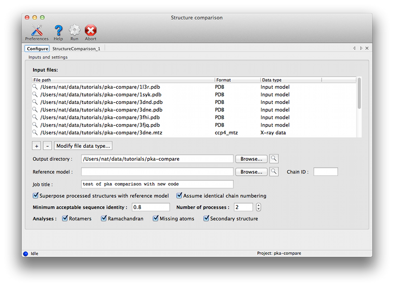 Currently the options for adding large numbers of files are limited. PDB files may be dragged into the list at the top of the window. If you have a directory containing multiple allowed file types, you may simply drag the directory in, and it will automatically guess the appropriate use for each file. If the PDB and reflection files use similar root filenames, or occur in pairs in the same directories, the association between them will be guessed automatically. For instance, the following pair of files will automatically be recognized as model and experimental data: 1syk.pdb 1syk.mtz while these will be recognized as model and map coefficients: 1syk.pdb 1syk_map_coeffs.mtz If the program does not automatically guess the associations correctly, you can manually specify which model goes with each reflections file. 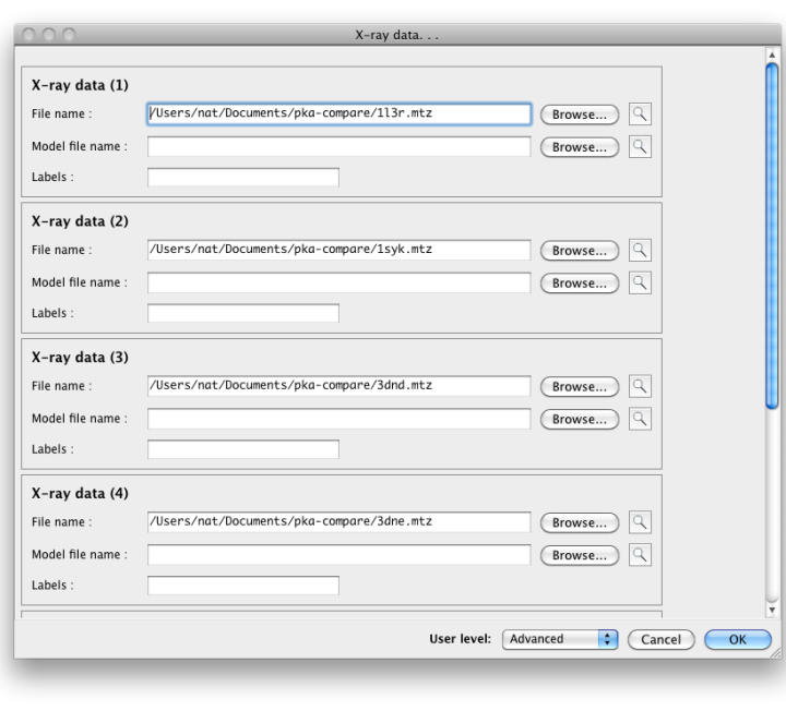 The map calculations have been parallelized, and this part of the program scales extremely well over multiple processors. The GUI will automatically be set to use NCPU - 1 processes, but you may reduce this if desired. The most important configurable option is the choice of superposing the models and maps prior for viewing together in Coot or PyMOL. This is very advantageous for comparing regions of difference, instead of switching between views for each chain. However, it has the drawback of removing the chains being analyzed from their original context, possibly obscuring other features that account for the observed structures. If you choose to turn on the superpositioning, the extracted chains will be written out as separate files in the results directory (along with reoriented maps for each chain, if available). Otherwise, the original models will be used for viewing. (Note that the analyses which depend on local environment in the crystal will still be run on the original models, and the coordinates mapped to their new positions.) In addition to the models actually being compared, you may also provide a "reference model" on which all other chains will be superposed. If you do not explicitly provide a reference model, the first chain found in the list of input files will be used instead. However, it may be advantageous to explicitly define this model if you are concerned about the quality or consistency of the structural alignments. Handling heterogeneous sequencesHomologous structures and insertion codes are now supported. To ensure that the residue numbering is interpreted correctly, you will need to uncheck the box labeled "Assume identical chain numbering". The sequence you provide as input will be used to pick out similar chains, which will then be aligned to the reference model. The numbering displayed in the output grids will reflect the residue IDs in the reference model; for residues present in other chains but not the reference model, the residue ID will be displayed as "--", but the residue name(s) will still be shown. The primary limitation at this point is the lack of any direct link back to the original residue IDs, but the models displayed in Coot and PyMOL preserve these IDs. ResultsAll output files will be written to a directory named StructureComparison_X (where X is the job ID). If you have turned on structure superpositioning, there will be a separate PDB file for each chain, plus CCP4 map files if map coefficients were available. If the map coefficients were calculated from input X-ray data (not pre-calculated) these will also be written out. When the application is finished running, a summary tab will show a list of all chains used for the analysis, with basic statistics. Additional tabs will be added for each analysis. Each tab contains a grid with chains organized one per row, and residues of interest in columns. Color coding indicates the relationship of the specific residue in each cell to the equivalent residues, and/or properties such as validation outlier or multiple conformations. Cells colored in grey indicated residues missing from the input chain. 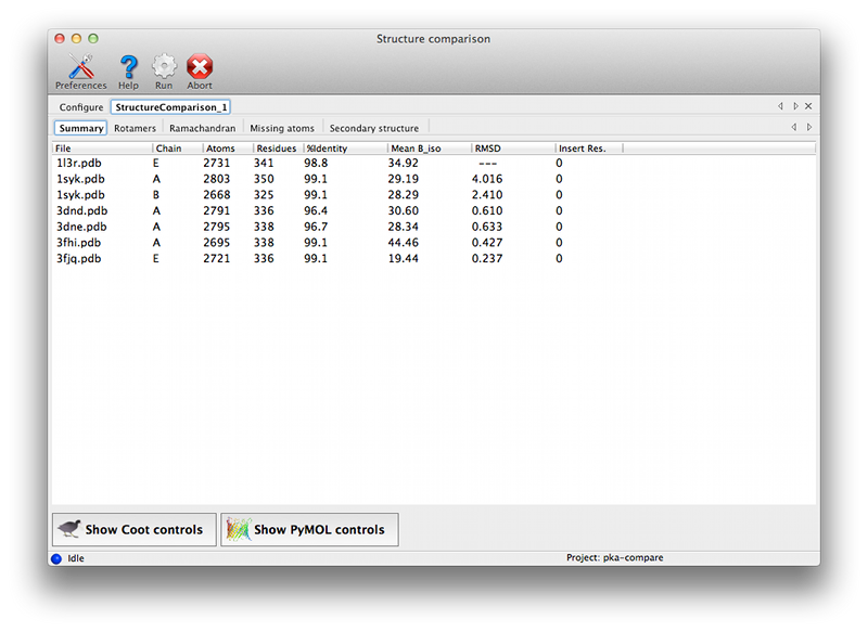 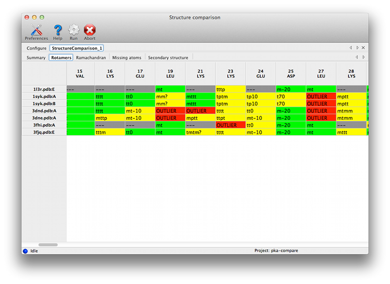 Both validation and unrelated atomic properties are included in the application; in theory, any analysis easily reduced to per-residue information can also be integrated. The criteria used to display results vary widely, but as the primary purpose of the program is to highlight regions of difference, homogeneous regions will usually be omitted from the grid.
 Interacting with CootTo show controls for sending data to and from Coot, click the icon on the toolbar of the results window. A small panel will appear: 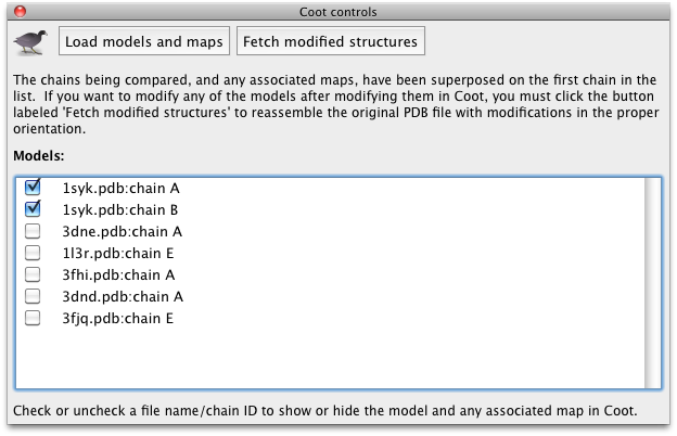 Click the button labeled "Load models and maps" to read all structures into Coot simultaneously. Once this is complete they will appear in a checklist in PHENIX; unchecking any structure will hide the associated objects in Coot. As with other validation programs in the PHENIX GUI, clicking on the field for any residue in the results grid will recenter Coot on that residue (in the appropriate frame of reference depending on whether models were superposed). You may now adjust the models to match a consensus if desired. 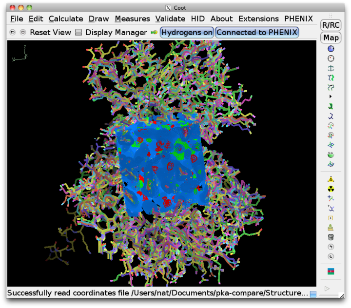 If the structures were superposed, you should not try to use the models in Coot for further refinement. Instead, click the button labeled "Fetch modified structures" to write out the models from Coot to the results directory. PHENIX will automatically recover the original orientation and replace the unmodified chain in the input structure with the model from Coot, while leaving all other atoms in place. The complete files will be written out to the result directory, renamed with the extension "_modified.pdb". References
| |